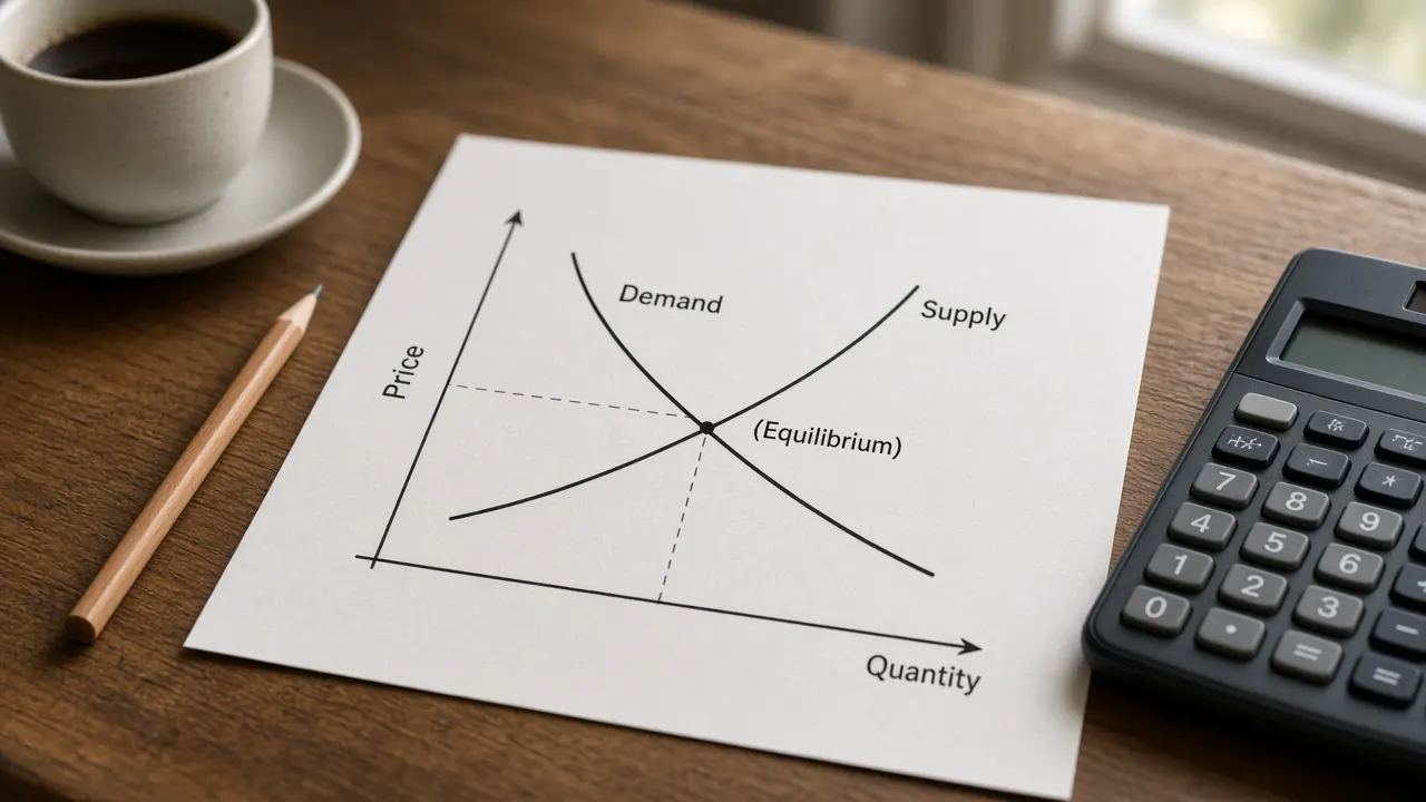
The aggregate demand and aggregate supply model shows how the price level and real GDP are set together. Aggregate demand is the spending households, firms, government, and the rest of the world plan at each price level, and it slopes down. Short run aggregate supply slopes up while some wages and prices are sticky, and long run aggregate supply is a vertical line at potential output.
Educational only, not investment advice. The graph uses invented index points so the arithmetic stays visible. It is not a reading of UK or US data, and it is not a forecast. For the building blocks, start with GDP, inflation, and monetary and fiscal policy. Short definitions sit in the glossary under aggregate demand, aggregate supply, and price level.
Demand shocks and supply shocks on the graph
Move aggregate demand, move short run aggregate supply, or open a preset. The readout states the new price level, real GDP, the output gap direction, and whether the price level shows inflation pressure or deflation pressure relative to the start. Potential real GDP stays at 100. Pale dashed lines, once a curve has moved, are the starting curves. The shaded band, when it appears, is the gap between real GDP and potential.
Vertical axis: price level. Horizontal axis: real GDP. AD is the downward line. SRAS is the upward line. LRAS is the vertical dashed line at potential output. Do not label these axes as price and quantity. Those words belong on a single market graph.
Arrow keys move a slider by 10 index points. The range runs from 40 points left of the start to 40 points right of the start. Right means more demand, or more short run supply.
What happened
Price level 100. Real GDP 100. Potential real GDP is 100. This is the starting equilibrium. Real GDP is at potential, so there is no output gap. The price level matches the starting equilibrium, so there is no inflation pressure and no deflation pressure.
The same scenarios are in the table, so the lesson is readable without the graph.
| Scenario | Aggregate demand | Short run aggregate supply | Price level | Real GDP | Reading |
|---|---|---|---|---|---|
| Starting equilibrium | Starting curve | Starting curve | 100 | 100 | At potential. No output gap. No inflation pressure and no deflation pressure. |
| Positive demand shock | Right by 20 | Starting curve | 110 | 110 | Inflationary gap and inflation pressure. Demand pull. |
| Negative demand shock | Left by 20 | Starting curve | 90 | 90 | Recessionary gap and deflation pressure. |
| Negative supply shock | Starting curve | Left by 20 | 110 | 90 | Stagflation. Recessionary gap and inflation pressure. Cost push. |
| Positive supply shock | Starting curve | Right by 20 | 90 | 110 | Inflationary gap, with deflation pressure, because the price level falls. |
| Recessionary gap self correction | Left by 20 | Right by 20 | 80 | 100 | Output back at potential, with deflation pressure. Before wages adjusted, real GDP was 90 and the price level was 90. |
Why aggregate demand slopes down
Aggregate demand is not the demand curve for one good. It is planned spending on domestic output at each price level: consumption, investment, government spending, and net exports. A higher price level goes with less of that spending. Three links, not a single product substitution story, explain the downward slope.
Wealth effect
People hold some wealth as money. When the price level rises, those balances buy fewer goods. Households feel poorer in real terms and cut consumption. When the price level falls, the same balances buy more, and consumption rises. Textbooks sometimes call this the real balances effect. The idea is the purchasing power of money people already hold.
Interest rate effect
A higher price level means households and firms need more cash to carry out the same real purchases. That extra demand for money pushes interest rates up. Higher interest rates discourage borrowing for investment and for some large household purchases, so planned spending falls. A lower price level eases that pressure. The rate that matters for the spending decision is a real rate, which is the idea on the real interest rates page. The real interest rate calculator is the arithmetic, with numbers you type. The graph that keeps the nominal rate and the real rate apart is the money market and the loanable funds market.
Exchange rate effect
If the domestic price level rises while foreign prices do not, home produced goods become more expensive relative to foreign goods. Exports fall and imports rise, so net exports fall. A lower domestic price level does the reverse. The international trade topic is the wider map, and exchange rates and purchasing power parity covers the rate itself. A change in the exchange rate for some other reason, such as a shift in capital flows, is a shift of aggregate demand, not a slide along it.
Hold those three links together. The price level changed, and you moved along aggregate demand. You did not draw a new curve.
Short run aggregate supply and long run aggregate supply
Aggregate supply is the output firms plan at each price level. The short run version and the long run version answer different questions, and exam graphs need both.
Why short run aggregate supply slopes up
In the short run, many wages and some other input prices are stuck in contracts, menus, and slow bargaining. Suppose the price level rises and a firm’s nominal wage has not yet changed. The wage is cheaper relative to the firm’s selling price, so producing more looks profitable. Output rises. If the price level falls while the wage is stuck, the real cost of labour is higher than the firm expected, and output falls. That is why short run aggregate supply slopes upward. Sticky wages are the usual classroom reason. Sticky prices in some firms, while others adjust, can produce the same slope.
A movement along short run aggregate supply is also the short run link between output and the price level. Higher output usually means more employment. The Phillips curve tells a related story with unemployment and inflation. The Phillips curve calculator is that second sketch. The two graphs are not the same object.
Why long run aggregate supply is vertical
Given time, contracts are rewritten. Wages and other input prices catch up to the price level. Firms no longer see a lasting profit from a higher price level alone, because costs have risen too. Output settles at what the economy can sustain with its labour, capital, technology, and institutions. That level is potential output. Long run aggregate supply is vertical there. Moving up or down the line changes the price level and leaves real GDP at potential.
Potential output is an estimate, not a scanner reading. The output gap page is about how economists compare actual GDP with that estimate, and why two careful estimates can disagree. This graph holds potential at 100 so the short run gaps stay easy to see. A lasting change in labour supply, the capital stock, or productivity would move the vertical line. The same lasting change shifts a production possibilities curve outward. That curve is the two good picture of capacity. This graph is the price level and real GDP picture. A temporary cost shock usually does not move either frontier.
What shifts aggregate demand
Aggregate demand shifts when one of its pieces changes for a reason other than the price level. The pieces are consumption (C), investment (I), government spending (G), and net exports (NX).
- Consumption. Stronger household confidence, higher wealth, or lower taxes that raise disposable income can lift consumption and shift aggregate demand right. The opposite shifts it left.
- Investment. More optimistic firms, or a lower interest rate that is not itself caused by the price level, raise investment and shift aggregate demand right. Pessimism or higher borrowing costs shift it left.
- Government spending. Higher government purchases of goods and services shift aggregate demand right. Lower purchases shift it left.
- Net exports. Stronger foreign income raises exports. A weaker home currency, if it makes exports cheaper and imports dearer, can raise net exports. Either can shift aggregate demand right. Weaker foreign income or a stronger home currency can shift it left.
Monetary policy and fiscal policy are the usual classroom reasons those pieces move. A lower policy rate, or in some episodes large scale asset purchases, supports interest sensitive spending and shifts aggregate demand right. A higher policy rate shifts it left. When the usual rate is already very low, some central banks have used bond purchases. That tool is quantitative easing, and it is not the same thing as a routine rate cut. Higher government spending or a tax cut that households spend shifts aggregate demand right. A spending cut or a tax increase shifts it left.
How large the output change is, for a given fiscal impulse, is the question on the fiscal multipliers page. The fiscal multiplier calculator runs a transparent classroom version. A multiplier is not a law, and it is not one for one in every setting. The wider map of who does what is the monetary and fiscal policy topic.
A change in the price level does not shift aggregate demand. It moves you along the curve you already drew.
What shifts short run aggregate supply
Short run aggregate supply shifts when the cost of producing a given level of output changes, or when productivity changes, at a given price level.
- Input prices. Higher wages, energy prices, or raw material prices shift short run aggregate supply left. Firms supply less real GDP at the same price level, or they require a higher price level to supply the same real GDP. Lower input prices shift the curve right.
- Productivity. If the same inputs produce more output, costs per unit fall and short run aggregate supply shifts right. A loss of productivity shifts it left. A permanent productivity gain can also shift long run aggregate supply right. This page keeps the vertical line fixed so you can see the short run move on its own.
- Supply shocks. A harvest failure, a disruption to energy, or a similar hit to production is a negative supply shock and shifts short run aggregate supply left. A favourable shock shifts it right. The glossary entry for a supply shock is the one line version.
Again, the price level itself is a movement along short run aggregate supply. If the only thing that changed is the price level, do not draw a new curve.
Recessionary gaps, inflationary gaps, and self correction
The short run equilibrium is the crossing of aggregate demand and short run aggregate supply. Compare that real GDP with potential, which is the long run line.
A recessionary gap means real GDP is left of potential. Labour and plant are underused. In the textbook self correction, weak demand for labour eventually lowers nominal wages and other flexible input prices. Costs fall, short run aggregate supply shifts right, and the economy slides along the existing aggregate demand curve. Real GDP returns to potential at a lower price level than the short run point, and often lower than the original equilibrium too.
An inflationary gap means real GDP is right of potential. Labour markets are tight. Nominal wages rise, short run aggregate supply shifts left, and real GDP returns to potential at a higher price level. Self correction of an inflationary gap adds inflation pressure. It does not cool the price level.
The percent version of that distance is the output gap: (real GDP minus potential) divided by potential. The output gap calculator does that percent with levels you type. A gap in real GDP usually shows up in unemployment as well. Okun's law is a rule of thumb from a GDP growth gap to a change in unemployment, and the Okun's law calculator is the arithmetic. Self correction can be slow. Nothing in the diagram says wages will fall quickly, or that policy should wait.
Demand pull inflation, cost push inflation, and stagflation
Demand pull inflation is a right shift of aggregate demand. In the short run the new crossing has a higher price level and higher real GDP. If the shift pushes output past potential, the gap is inflationary. Later wage adjustment can shift short run aggregate supply left and raise the price level further, with output back at potential. The inflation started from spending.
Cost push inflation is a left shift of short run aggregate supply. The new crossing has a higher price level and lower real GDP. Output is weak and the price level is up. That pairing is stagflation. A negative demand shock is a different picture: output falls and the price level falls. If a graph shows a lower price level, do not call it stagflation.
The negative supply shock button draws stagflation. The positive demand shock button draws demand pull. Use the two presets side by side and read the price level, not only real GDP. The inflation topic is about how a price index is measured once you leave the classroom axes. A price index such as CPI or PCE is one way statistical agencies summarise the price level. The model here uses an index point you can shift, not a live print.
How policy responds
Policy in this model usually shifts aggregate demand. It can also, more slowly, aim at aggregate supply.
In a recessionary gap, expansionary fiscal policy (higher government spending or lower taxes) or expansionary monetary policy (a lower policy rate, and in some episodes asset purchases) shifts aggregate demand right, toward potential. Compared with waiting for self correction, that path returns output to potential at a higher price level. The wage decline, and the extra fall in the price level, need not happen. The cost is that you give up some of the disinflation self correction would have produced.
In an inflationary gap, contractionary fiscal or monetary policy shifts aggregate demand left, toward potential, at a lower price level than self correction would reach. Waiting instead lets wages rise and short run aggregate supply shift left, which brings output back to potential and pushes the price level up. A simple guideline that raises a suggested policy rate when the output gap is positive is the Taylor rule. It is a classroom benchmark, not a description of the next decision.
Stagflation is the awkward case. Shifting aggregate demand right can close the recessionary gap, but it raises the price level further. Shifting aggregate demand left can fight the inflation, but it deepens the output loss. A policy that lowers costs or raises productivity shifts short run aggregate supply right, which can lift output and ease the price level together. That is slower and less certain than a rate move. The diagram shows the dilemma. It does not pick a side.
None of these arrows is a recommendation to change a tax, a spending bill, or a policy rate. Read the monetary and fiscal policy topic for who holds which tool in the UK and the US, and primary sources for any real decision.
A worked example
The graph uses straight lines and invented index points. Potential real GDP is 100. A demand shift is positive when aggregate demand moves right. A supply shift is positive when short run aggregate supply moves right.
Aggregate demand: price level = 200 plus the demand shift, minus real GDP.
Short run aggregate supply: price level = real GDP minus the supply shift.
Real GDP = (200 plus the demand shift plus the supply shift) divided by 2.
Price level = (200 plus the demand shift minus the supply shift) divided by 2.
Starting point. Both shifts are 0. Real GDP = 200 divided by 2 = 100. The price level = 200 divided by 2 = 100. Output is at potential. There is no output gap, and no inflation pressure or deflation pressure relative to this start. Check the supply line: price level = 100 minus 0 = 100. The two lines agree.
Positive demand shock. The demand shift is 20 and the supply shift is 0. Real GDP = (200 plus 20 plus 0) divided by 2 = 110. The price level = (200 plus 20 minus 0) divided by 2 = 110. The output gap is (110 minus 100) divided by 100, which is 10 percent of potential. That is an inflationary gap, and the price level is higher, so the sketch shows inflation pressure. This is demand pull.
Negative supply shock. The demand shift is 0 and the supply shift is minus 20, which is a left move. Real GDP = (200 plus 0 plus minus 20) divided by 2 = 90. The price level formula subtracts the supply shift, and subtracting a supply shift of minus 20 adds 20, so the price level is (200 plus 20) divided by 2 = 110. The output gap is (90 minus 100) divided by 100, which is minus 10 percent of potential. That is a recessionary gap with a higher price level: stagflation, and cost push inflation pressure.
Self correction after a negative demand shock. First the demand shift is minus 20 and the supply shift is 0. Real GDP = 90 and the price level = 90. That is the hollow dot on the self correction preset: a recessionary gap with deflation pressure. Then nominal wages ease and the supply shift becomes plus 20, while demand stays at minus 20. Real GDP = (200 minus 20 plus 20) divided by 2 = 100. The price level = (200 minus 20 minus 20) divided by 2 = 80. Output is back at potential. The price level is lower than both the original 100 and the short run 90. Policy could instead have put the demand shift back to 0 and left supply at 0, which returns real GDP to 100 at a price level of 100. Same output, different price level.
Type 110 and 100 into the output gap calculator and you should see plus 10 percent. Type 90 and 100 and you should see minus 10 percent. Those are the gaps in this example. They are not a claim about current GDP.
Common AP exam mistakes
AP Macroeconomics Unit 3, national income and price determination, is where this model is taught. The names in this section follow the public course description. This page is not an official exam item and it is not affiliated with the College Board.
- Movement along, versus a shift. A change in the price level slides you along aggregate demand and along short run aggregate supply. A new curve needs something else: confidence, policy, foreign income, input prices, productivity, or a supply shock. If your explanation of a shift is only “prices rose,” the curve did not shift.
- Axes. Label the vertical axis price level and the horizontal axis real GDP. Price and quantity are the axes of one market, as on the supply and demand topic and the supply and demand calculator. Real GDP is not the quantity of a single good, and the price level is not the price of that good.
- The long run line. Long run aggregate supply is vertical at potential. It does not slope up. A higher price level does not move it. Do not use one label for both short run and long run aggregate supply.
- Which curve moved. Stagflation is a left shift of short run aggregate supply. A left shift of aggregate demand lowers the price level. Right is more demand or more short run supply. Left is less.
- What self correction moves. Self correction shifts short run aggregate supply. It does not shift aggregate demand, and it does not shift long run aggregate supply. In a recessionary gap the short run curve moves right. In an inflationary gap it moves left.
- Gap versus the price level. An inflationary gap means real GDP is above potential. It does not, by itself, mean the price level just rose. A positive supply shock can raise real GDP above potential and lower the price level in the same move. Read both numbers.
Common questions
What is the aggregate demand and aggregate supply model?
The aggregate demand and aggregate supply model is the classroom picture of how the price level and real GDP are determined together. Aggregate demand is planned spending at each price level. Short run aggregate supply is planned output while some wages and prices are sticky. Long run aggregate supply is vertical at potential output. The short run equilibrium is where aggregate demand crosses short run aggregate supply. It is a teaching model, not a forecast and not investment advice.
Why does aggregate demand slope downward?
Aggregate demand slopes downward because a higher price level reduces planned spending. The wealth effect means the money people already hold buys less, so consumption falls. The interest rate effect means households and firms need more cash for the same purchases, which pushes interest rates up and reduces spending that is sensitive to the interest rate. The exchange rate effect means domestic goods become more expensive relative to foreign goods, so net exports fall. A lower price level works in the opposite direction. A change in the price level is a movement along the curve, not a shift.
What is the difference between short run and long run aggregate supply?
Short run aggregate supply slopes upward because many wages and some prices are sticky. A higher price level, before costs have fully adjusted, makes extra production look profitable, so real GDP rises. Long run aggregate supply is vertical at potential output. Once wages and other input prices catch up, output depends on labour, capital, and technology, not on the price level. A higher price level moves the economy up the vertical line. It does not move the line.
What shifts aggregate demand?
Aggregate demand shifts when spending changes for a reason other than the price level. The pieces are consumption, investment, government spending, and net exports. Expansionary monetary policy or expansionary fiscal policy shifts aggregate demand to the right. Contractionary policy shifts it to the left. Confidence, wealth, foreign income, and the exchange rate can shift it too. A change in the price level is a movement along aggregate demand, not a shift.
What shifts short run aggregate supply?
Short run aggregate supply shifts when production costs or productivity change. Higher wages, energy prices, or other input prices shift it left. Lower input prices shift it right. Weaker productivity shifts it left. Stronger productivity shifts it right. A negative supply shock, such as a disruption to energy, shifts it left and can produce stagflation. A change in the price level is a movement along the curve, not a shift.
What is the difference between a recessionary gap and an inflationary gap?
A recessionary gap means short run equilibrium real GDP is to the left of long run aggregate supply, so output is below potential. An inflationary gap means real GDP is to the right of long run aggregate supply, so output is above potential. In the classroom self correction, wages and other input prices adjust and short run aggregate supply shifts until output returns to potential. Policy can instead shift aggregate demand. The two paths do not end at the same price level.
What does stagflation look like on an AD AS graph?
Stagflation is weak output together with a higher price level. On the graph it is a left shift of short run aggregate supply. Real GDP falls and the price level rises. A left shift of aggregate demand is not stagflation, because that shock lowers the price level. The negative supply shock control on this page draws the stagflation case. It is a teaching sketch, not a claim about any particular year.
Nothing on this page is a recommendation to buy, sell, or hold any security, currency, or derivative, or to choose a tax, a spending bill, or an interest rate. Educational macro literacy is the only goal.
Sources
- OpenStax, Principles of Macroeconomics 3e, section 11.2, Building a Model of Aggregate Demand and Aggregate Supply
- OpenStax, Principles of Macroeconomics 3e, section 11.3, Shifts in Aggregate Supply
- OpenStax, Principles of Macroeconomics 3e, section 11.4, Shifts in Aggregate Demand
- OpenStax, Principles of Macroeconomics 3e, section 11.5, How the model incorporates growth, unemployment, and inflation
- College Board, AP Macroeconomics course page (Unit 3, national income and price determination, as course context only)
- College Board, AP Macroeconomics Course and Exam Description (Unit 3)
- Board of Governors of the Federal Reserve System, monetary policy goals and how policy works
- Board of Governors of the Federal Reserve System, Monetary Policy
- Bureau of Economic Analysis, Gross Domestic Product