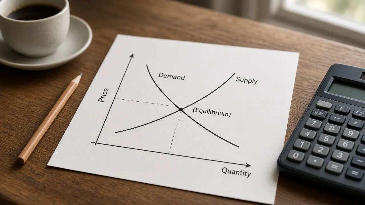
The money market graph shows how the nominal interest rate is set. Money supply is a vertical line, because in this classroom model the central bank sets the stock of money. Money demand slopes down, because a higher nominal interest rate raises the opportunity cost of holding money. The crossing is the nominal interest rate.
The loanable funds market shows how the real interest rate is set. The supply of loanable funds slopes up, because a higher real rate draws out saving. The demand for loanable funds slopes down, because a higher real rate discourages borrowing. The crossing is the real interest rate and the flow of funds lent during a period.
The key difference is the axis and the object. The money market is a stock of money and a nominal rate. The loanable funds market is a flow of saving and borrowing and a real rate. A government deficit raises the real rate and crowds out some private borrowing. An open market purchase shifts money supply to the right and lowers the nominal rate. An open market sale shifts money supply to the left and raises the nominal rate.
Educational only, not investment advice. Both graphs use invented index points so the arithmetic stays visible. They are not a reading of UK or US data, and they are not a forecast. The policy map is monetary and fiscal policy. How the Fed sets its rate with plentiful reserves is the reserve market. The open economy version is the foreign exchange market. What the stock of money includes is M1 and M2. How a nominal rate becomes a real rate is real interest rates. Short definitions sit in the glossary under loanable funds market, crowding out, nominal, real interest rate, and M1.
Shocks on the two graphs
Each control moves one market. An open market purchase or sale shifts money supply. Higher income shifts money demand. A larger government deficit shifts demand for loanable funds. Higher private saving shifts supply of loanable funds. Pale dashed lines, once a curve has moved, are the starting curves. The readout under each graph states the new equilibrium. The other graph stays where you left it.
Money market
Vertical axis: nominal interest rate, in percent. Horizontal axis: quantity of money, an invented index. MS is the vertical line. MD is the downward line. Do not put the real interest rate on this graph.
Arrow keys move a slider by 10 index points. Right means a larger money supply, or more money demanded at each nominal rate. The range runs from 30 points left of the start to 30 points right of the start.
What happened
Nominal interest rate 6 percent. Quantity of money 100. This is the starting money market. Money supply is vertical at a quantity of 100. Money demand slopes down. The loanable funds curves are a separate graph and do not move with this control.
Loanable funds market
Vertical axis: real interest rate, in percent. Horizontal axis: quantity of loanable funds, an invented flow. DLF slopes down. SLF slopes up. Do not put the nominal interest rate on this graph. The 6 percent start on the money market and the 4 percent start here are separate sketches, not a Fisher calculation.
Arrow keys move a slider by 10 index points. Right means more government borrowing, or more private saving. The range runs from 40 points left of the start to 40 points right of the start.
What happened
Real interest rate 4 percent. Quantity of loanable funds 100. Private borrowing 100. This is the starting loanable funds market. Supply slopes up and demand slopes down. Private borrowing matches the equilibrium quantity because the deficit shift is zero. The money market curves do not move with this control.
The same scenarios are in the tables, so the lesson is readable without the graphs.
| Scenario | Money supply | Money demand | Nominal interest rate | Quantity of money |
|---|---|---|---|---|
| Starting equilibrium | Vertical at 100 | Starting curve | 6 percent | 100 |
| Open market purchase | Right by 20 | Starting curve | 4 percent | 120 |
| Open market sale | Left by 20 | Starting curve | 8 percent | 80 |
| Higher income | Vertical at 100 | Right by 20 | 8 percent | 100 |
| Scenario | Demand | Supply | Real interest rate | Quantity of funds | Private borrowing |
|---|---|---|---|---|---|
| Starting equilibrium | Starting curve | Starting curve | 4 percent | 100 | 100 |
| Government deficit increase | Right by 40 | Starting curve | 6 percent | 120 | 80 |
| Higher private saving | Starting curve | Right by 40 | 2 percent | 120 | 120 |
| Deficit drawn as less public saving | Starting curve | Left by 40 | 6 percent | 80 | 80 |
The money market
The money market in this course is not the market for a single bond and it is not the loanable funds market with the labels swapped. The vertical axis is the nominal interest rate. The horizontal axis is the quantity of money, a stock measured at a point in time. M1 and M2 are two US cuts of that stock. The M1 and M2 explainer is about what each cut includes. This graph does not pick M1 or M2. It only needs a quantity the central bank can shift.
Why money demand slopes down
Money is useful for payments, and it usually pays little or no interest compared with a bond. The nominal interest rate is the opportunity cost of holding money instead of that bond. When the nominal rate rises, people and firms try to hold less money and more interest bearing assets. When the nominal rate falls, the cost of holding money is lower, so the quantity of money demanded rises. That is a movement along money demand. You do not draw a new curve just because the rate changed.
What shifts money demand
Money demand shifts when people want a different quantity of money at the same nominal rate.
- Income. Higher income means more transactions, so money demand shifts right and the nominal rate rises. Lower income shifts money demand left and the nominal rate falls. The higher income button is this case.
- The price level. A higher price level means the same real purchases need more cash. Money demand shifts right. A lower price level shifts it left. On the aggregate demand and aggregate supply graph, this link is one reason aggregate demand slopes down: a higher price level raises money demand, the nominal rate rises, and interest sensitive spending falls.
- Not an open market operation. A central bank purchase or sale changes the stock of money. That is money supply, not money demand.
Why money supply is vertical
In the classroom drawing the central bank chooses the quantity of money, and that quantity does not depend on the nominal rate. The curve is vertical. A higher rate moves you along money demand until people are content to hold the stock that exists. It does not slide you along a sloping money supply.
That vertical line is an exam picture, not a full account of how the Federal Reserve or the Bank of England operates in an ample reserves system. The Fed describes open market operations as buying and selling securities in the open market. In recent years it has also steered the federal funds rate with administered rates, including interest on reserve balances, rather than by keeping reserves scarce every day. The money multiplier calculator is the separate classroom story about required reserve ratios and deposit expansion. A required reserve ratio of zero does not make this vertical line a live policy rule. Use the graph for the nominal rate logic. Do not treat it as a forecast of the next policy decision. The policy rate entry is the short name for the rate a central bank sets or targets.
The loanable funds market
Loanable funds are saving made available for borrowers to use. The vertical axis is the real interest rate. The horizontal axis is a flow: funds per period, not a stock of money sitting in a vault. Supply slopes up because a higher real rate makes saving more attractive. Demand slopes down because a higher real rate makes borrowing for investment, and for other interest sensitive spending, less attractive. The glossary entry is loanable funds market.
In a closed economy with no international borrowing, national saving is private saving plus public saving. Public saving is tax revenue minus government spending. A budget surplus is positive public saving. A fiscal deficit is negative public saving. The real rate settles where the flow of saving equals the flow of borrowing. The real interest rates page is the Fisher arithmetic that links this real rate to a nominal quote. The real interest rate calculator does that subtraction with numbers you type. It does not draw these curves.
The Bureau of Economic Analysis publishes a personal saving rate and government receipts and expenditures. Those releases are the measured cousins of private saving and the deficit. This page does not download them. The sliders are not those series.
Open market operations and the nominal rate
An open market purchase means the central bank buys bonds and pays the sellers, which adds reserves. In the classroom money market the money supply shifts right, the nominal interest rate falls, and the quantity of money rises. An open market sale pulls reserves in, shifts money supply left, and raises the nominal interest rate. The purchase and sale buttons use a shift of 20 on the invented scale: the nominal rate moves from 6 percent to 4 percent, or from 6 percent to 8 percent. The quantity of money moves from 100 to 120, or from 100 to 80.
Those buttons do not shift money demand, and they do not shift the loanable funds curves. In this simple split, the central bank changes the nominal rate in the money market. The real rate in the loanable funds market is about saving and investment. Mixing the two graphs is the usual exam error.
Higher income is the other money market button. Money demand shifts right by 20, the nominal rate rises from 6 percent to 8 percent, and the quantity of money stays at 100 because the vertical supply did not move. People want to hold more money. The fixed stock only clears at a higher opportunity cost.
Large scale asset purchases, often called quantitative easing, are also bond buying, usually when the short policy rate is already very low and the aim is longer term yields. That tool is quantitative easing. It is related to an open market purchase and it is not the same classroom arrow as a routine shift of a vertical money supply line.
Deficits, private saving, and crowding out
Crowding out is the idea that government borrowing raises the real interest rate and reduces interest sensitive private spending. The College Board course framework asks students to show that with the loanable funds market. Two drawings are both taught. The real rate rises in both. The quantity you read off the horizontal axis does not.
Deficit as a right shift of demand
Treat the government as one more borrower. Demand for loanable funds shifts right. On this page the deficit button shifts demand right by 40. The real rate rises from 4 percent to 6 percent. The equilibrium quantity of funds rises from 100 to 120, because the higher real rate draws out more saving. Private borrowing falls from 100 to 80. The extra government borrowing is 40, and 20 of the funds that private borrowers used to take are now too expensive for them. That 20 is the crowding out in this drawing. Total funds can rise while private investment falls. If an answer says the equilibrium quantity fell, it is using the other drawing.
Deficit as a left shift of supply
National saving is private saving plus public saving. A deficit reduces public saving, so the supply of loanable funds shifts left. The last row of the table is that drawing: supply left by 40, demand unchanged. The real rate again rises from 4 percent to 6 percent. The equilibrium quantity falls from 100 to 80. In this drawing the quantity on the axis is private investment, so crowding out is the smaller quantity itself. The deficit button does not draw this case. The supply left control does. Either drawing is acceptable when the curve you shift matches the story you tell. Shifting both curves for one deficit double counts it.
Higher private saving
Higher private saving shifts supply right. The saving button shifts supply right by 40. The real rate falls from 4 percent to 2 percent and the quantity of funds rises from 100 to 120. Private borrowing rises with it, because the deficit shift is zero. This is not a money supply shift. Households saving more does not, by itself, print a larger stock of money.
How large the output effect of a deficit is, after crowding out, is the question on the fiscal multipliers page. A simple spending multiplier from the marginal propensity to consume ignores the real rate. Crowding out is one reason estimated multipliers are often smaller than that sketch. The fiscal multiplier calculator is the arithmetic without this graph.
From these graphs to aggregate demand
The aggregate demand and aggregate supply model is the next picture, with the price level and real GDP. These two graphs are how the course explains the interest rate piece of that picture.
An open market purchase lowers the nominal rate in the money market. Lower borrowing costs support interest sensitive consumption and investment, so aggregate demand shifts right. An open market sale does the reverse. The size of any deposit expansion behind that money stock is the money multiplier sketch, not a second shift of aggregate demand.
A deficit has two pushes. Government purchases of goods and services shift aggregate demand right. Government borrowing raises the real rate in the loanable funds market and crowds out some private investment, which shifts aggregate demand back left by part of that gain. The net shift can still be to the right. It is smaller than the government spending arrow alone. That partial offset is why a fiscal multiplier and a loanable funds graph belong in the same answer.
Nothing here says a finance ministry should run a deficit or a central bank should buy bonds. The graphs show directions. Primary sources, not this page, describe any real decision.
A worked example
The graphs use straight lines and invented numbers. Shifts are in index points. A positive money supply shift is a right move. A positive money demand shift is a right move. A positive deficit shift is extra government borrowing, drawn as a right move of demand. A positive saving shift is a right move of supply.
Nominal interest rate = (60 + money demand shift minus money supply shift) divided by 10.
Quantity of money = 100 + money supply shift.
Quantity of loanable funds = (200 + deficit shift + saving shift) divided by 2.
Real interest rate = (140 + deficit shift minus that quantity) divided by 10.
Private borrowing = quantity of loanable funds minus the deficit shift.
Money market start. Both shifts are 0. Quantity of money = 100. Nominal rate = 60 divided by 10 = 6 percent. Check money demand: at a quantity of 100 the rate on the starting demand line is (160 minus 100) divided by 10 = 6. The vertical supply and the demand line agree.
Open market purchase. Money supply shift is 20 and money demand shift is 0. Quantity = 120. Nominal rate = (60 minus 20) divided by 10 = 4 percent. The rate fell and the stock of money rose.
Open market sale. Money supply shift is minus 20 and money demand shift is 0. Quantity = 80. Nominal rate = (60 minus a supply shift of minus 20) divided by 10. Subtracting a negative number adds, so the rate is (60 + 20) divided by 10 = 8 percent.
Higher income. Money demand shift is 20 and money supply shift is 0. Quantity stays 100. Nominal rate = (60 + 20) divided by 10 = 8 percent. The stock did not change. The rate did.
Loanable funds start. Deficit shift and saving shift are 0. Quantity = 200 divided by 2 = 100. Real rate = (140 minus 100) divided by 10 = 4 percent. Private borrowing = 100 minus 0 = 100.
Government deficit, demand shift. Deficit shift is 40 and saving shift is 0. Quantity = (200 + 40) divided by 2 = 120. Real rate = (140 + 40 minus 120) divided by 10 = 6 percent. Private borrowing = 120 minus 40 = 80. Private borrowing fell by 20 even though total funds rose by 20. That is crowding out in the demand drawing.
The same deficit as less public saving. Leave demand at 0 and set the saving shift to minus 40, a left move of supply. Quantity = (200 minus 40) divided by 2 = 80. Real rate = (140 minus 80) divided by 10 = 6 percent. The real rate rose by the same 2 points. The quantity fell to 80, and in this drawing that quantity is private investment. Do not add this left shift on top of the demand shift of 40. That would count one deficit twice.
Higher private saving. Saving shift is 40 and deficit shift is 0. Quantity = 120. Real rate = (140 minus 120) divided by 10 = 2 percent. Private borrowing = 120. The real rate fell because more saving was offered at each rate.
The 6 percent nominal start and the 4 percent real start are not a statement that expected inflation is 2 percent. To subtract an inflation rate from a nominal rate you choose, use the real interest rate calculator.
Common AP exam mistakes
AP Macroeconomics Unit 4, the financial sector, teaches the money market and the loanable funds market. Unit 5, long run consequences of stabilization policies, teaches crowding out. The names follow the public course description. This page is not an official exam item and it is not affiliated with the College Board.
- Nominal versus real. The money market vertical axis is the nominal interest rate. The loanable funds vertical axis is the real interest rate. Swapping them is a different model.
- Stock versus flow. The money market horizontal axis is a stock of money. The loanable funds horizontal axis is a flow of saving and borrowing. M1 is not a quantity of loanable funds.
- The money supply slope. In this model money supply is vertical. A higher nominal rate does not move it. Do not draw money supply sloping up like the supply of loanable funds.
- Which curve the shock moves. An open market purchase or sale shifts money supply. Higher income or a higher price level shifts money demand. A change in the nominal rate, by itself, is a movement along money demand.
- One deficit, one shift. A deficit is either more government borrowing (demand right) or less public saving (supply left). The real rate rises either way. Shifting both curves counts the deficit twice. In the demand drawing, total funds can rise while private borrowing falls. In the supply drawing, the equilibrium quantity falls.
- Which market the central bank moves. An open market operation shifts the money market. It does not, in this simple split, shift saving or investment in the loanable funds market. A deficit shifts loanable funds. It does not shift the vertical money supply line.
- Axes from the wrong graph. Price and quantity belong on one market, as on the supply and demand topic. Price level and real GDP belong on aggregate demand and aggregate supply. These two graphs use an interest rate and either money or loanable funds.
Common questions
What is the difference between the money market and the loanable funds market?
The money market shows the stock of money and the nominal interest rate. Money supply is vertical and money demand slopes down. The loanable funds market shows the flow of saving and borrowing and the real interest rate. Supply of loanable funds slopes up and demand slopes down. The key difference is nominal versus real, and a stock of money versus a flow of saving. The graphs are a teaching model, not a forecast and not investment advice.
Why is the money supply curve vertical?
In this classroom model the central bank sets the quantity of money, so the money supply does not slope with the nominal interest rate. A higher nominal rate does not, by itself, create more money. An open market purchase or sale shifts the vertical line. A change in the nominal rate is a movement along money demand, not a shift of money supply.
What happens in the money market when the central bank buys bonds?
An open market purchase shifts the money supply to the right. The equilibrium nominal interest rate falls, and the quantity of money rises. An open market sale does the opposite: money supply shifts left and the nominal interest rate rises. This page's purchase button uses a right shift of 20 on an invented scale. It is not a reading of a Federal Reserve release.
How does higher income change the money market?
Higher income raises the transactions demand for money, so money demand shifts right. The nominal interest rate rises. The money supply curve stays put, so the quantity of money does not change unless the central bank shifts it. A higher price level can shift money demand the same way. The income button on this page is that right shift.
How does a government deficit cause crowding out?
A deficit means the government borrows. On this page that is a right shift of the demand for loanable funds. The real interest rate rises, and interest sensitive private borrowing falls. That fall in private spending is crowding out. You can draw the same deficit as a left shift of the supply of loanable funds, because public saving falls and national saving is public saving plus private saving. The real interest rate rises in that drawing too. The deficit button uses the demand shift.
What does higher private saving do to the real interest rate?
Higher private saving shifts the supply of loanable funds to the right. The real interest rate falls, and the equilibrium quantity of loanable funds rises. This is not a shift of money supply. Saving is a flow of funds over a period. The money supply is a stock.
Do the two graphs use the same interest rate?
No. The money market uses the nominal interest rate. The loanable funds market uses the real interest rate. A nominal rate is approximately a real rate plus expected inflation, which is the Fisher relation on the real interest rates page. The starting numbers on this simulator are separate invented sketches. They are not a claim that expected inflation equals the gap between them.
Nothing on this page is a recommendation to buy, sell, or hold any security, currency, or derivative, or to choose a tax, a spending bill, or an interest rate. Educational macro literacy is the only goal.
Sources
- College Board, AP Macroeconomics course page (Unit 4, the financial sector, and Unit 5, long run consequences of stabilization policies, as course context only)
- College Board, AP Macroeconomics Course and Exam Description (money market, loanable funds market, and crowding out)
- Board of Governors of the Federal Reserve System, Open Market Operations
- Board of Governors of the Federal Reserve System, monetary policy goals and how policy works
- OpenStax, Principles of Macroeconomics 3e, section 4.2, Demand and Supply in Financial Markets
- OpenStax, Principles of Macroeconomics 3e, section 15.3, How a Central Bank Executes Monetary Policy
- Bureau of Economic Analysis, Government Receipts and Expenditures
- Bureau of Economic Analysis, Personal Saving Rate