A production possibilities curve shows the most an economy can produce of two goods when it uses its resources fully and with the best methods it has. The slope is the opportunity cost: how much of one good you give up to make one more unit of the other. A curve that bows out, away from the origin, means that cost rises as you make more of one good. A straight line means the cost stays the same. Another name for the same picture is the production possibilities frontier.
A point on the curve is efficient. A point inside the curve is inefficient, because labour or capital is sitting idle, so the economy could make more without a new resource. A point outside the curve is unattainable until resources grow or technology improves. That outside point is not unemployment. Unemployment is the inside point.
The curve is the classroom picture of scarcity. Resources are limited, so a choice to have more of one good is a choice to have less of something else. Educational only, not investment advice, and not a recommendation about how many capital goods a country should build. The numbers on the graph are invented so the arithmetic stays visible. They are not UK or US production statistics and they are not a forecast. The study map is the AP Macroeconomics hub, Unit 1. The two good arithmetic for a straight line is the opportunity cost and comparative advantage calculator. Short definitions sit in the glossary under opportunity cost and comparative advantage.
Move a point and shift the curve
The graph starts as a bowed curve. Capital goods are on the vertical axis and consumer goods are on the horizontal axis. The along slider moves the mix from all capital goods to all consumer goods. The resource use slider pulls the point in toward the origin, which puts it inside the curve, or pushes it out past the starting curve, which makes it unattainable until you grow capacity. The curve size slider shifts the whole frontier outward or inward by the same percent on both axes. A dashed curve, once the size has changed, is the starting frontier. The straight line button swaps in constant opportunity cost. The readout under the controls states the two quantities, the opportunity cost on the curve at that mix, and whether the point is efficient, inefficient, or unattainable.
Vertical axis: capital goods, an invented index from 0 to 120. Horizontal axis: consumer goods, an invented index from 0 to 150. The shaded region is attainable. The solid curve is the current frontier. A dashed curve, when it appears, is the starting frontier. Do not put price and quantity on these axes.
Arrow keys move a slider by 5. The along slider runs from all capital goods to all consumer goods. Resource use and curve size each run from 70 percent to 130 percent of the start. The point is on the curve when resource use matches curve size. It is inside when resource use is lower, and outside when resource use is higher.
What happened
Consumer goods 50. Capital goods 60. This point is on the curve, so it is efficient. Making more of one good means giving up some of the other. The opportunity cost of 1 more consumer good is 0.8 capital goods. The opportunity cost of 1 more capital good is 1.25 consumer goods. The curve is bowed out, so that cost rises as you move toward more consumer goods. The curve is at its starting size.
The same cases are in the table, so the lesson is readable without the graph. Every row uses the formulas in the worked example.
| Case | Shape | Mix | Resource use | Curve size | Consumer goods | Capital goods | Status | Opportunity cost |
|---|---|---|---|---|---|---|---|---|
| On the curve | Bowed | 50 | 100 | 100 | 50 | 60 | Efficient | 0.8 |
| More consumer goods | Bowed | 80 | 100 | 100 | 80 | 28.8 | Efficient | 1.28 |
| More capital goods | Bowed | 20 | 100 | 100 | 20 | 76.8 | Efficient | 0.32 |
| Inside the curve | Bowed | 50 | 80 | 100 | 40 | 48 | Inefficient | 0.8 on the curve |
| Outside the curve | Bowed | 50 | 120 | 100 | 60 | 72 | Unattainable | 0.8 on the curve |
| Curve outward | Bowed | 50 | 100 | 120 | 50 | 60 | Inefficient | 0.8 |
| Curve inward | Bowed | 50 | 100 | 80 | 50 | 60 | Unattainable | 0.8 |
| Straight line | Straight | 50 | 100 | 100 | 50 | 40 | Efficient | 0.8 everywhere |
What the curve is
Draw two goods. This page uses consumer goods and capital goods, which is a common classroom pair, because the choice between them is also a choice about the future. Any other pair works if you can state what you give up: wheat and cotton, cars and computers, health care and education. The curve connects the combinations that fully use today's resources and today's methods.
Four assumptions sit under the drawing.
- Two goods. A real economy makes thousands of things. The picture keeps two so the tradeoff is visible. Adding a third good would need a third axis.
- Fixed resources. Labour, capital, and natural resources are held still while you move along one curve. A change in those resources is a new curve, not a slide along the old one.
- Fixed technology. The methods of production stay put along one curve. A better method is an outward shift, or a pivot if it helps only one good.
- Full use on the curve. Points on the curve mean resources are employed in production. Points inside mean some resource is idle or used in a wasteful way.
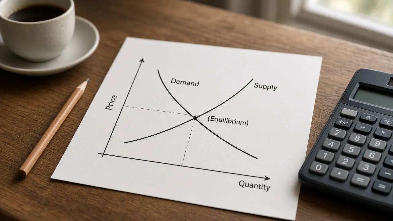
Scarcity is why the curve exists. Wants exceed what the resources can produce, so the economy cannot be at every point a person might like. The curve is the boundary. Supply and demand is a different picture: one market, with a price and a quantity. This graph has no price axis.
Opportunity cost and the slope
Opportunity cost is the next best thing you give up when you choose. On this graph the next best thing is the other good. If capital goods are on the vertical axis, a move to the right is more consumer goods, and the drop in the curve is the capital goods you no longer produce. That drop, per extra consumer good, is the opportunity cost of consumer goods.
Read the slope with the axes in mind. A steeper drop, more capital goods given up per step toward consumer goods, means a higher opportunity cost of consumer goods. A flatter stretch means a lower opportunity cost of consumer goods. The opportunity cost of capital goods is the reciprocal. If 1 consumer good costs 0.8 capital goods, then 1 capital good costs 1.25 consumer goods. Students who report the slope as the cost of the vertical good have the two costs swapped.
The cost is a marginal cost, the cost of one more unit at that point, not the cost of the entire pile of consumer goods. On a bowed curve the marginal cost changes as you move. On a straight line it does not. The opportunity cost calculator divides two maximum outputs, which is the straight line version of this slope.
Increasing and constant opportunity cost
Most production possibilities curves in this course bow out from the origin. The reason is increasing opportunity cost. Resources are not equally good at every job. The first consumer goods you add can use the labour and land that were least useful as capital goods, so you give up very little capital goods output. Later consumer goods have to pull in resources that were very good at making capital goods, so each extra consumer good costs more capital goods than the one before it. The curve gets steeper as you move toward consumer goods. That pattern is the law of increasing opportunity cost.
A straight line means constant opportunity cost. Every extra consumer good costs the same number of capital goods, from the first unit to the last. That drawing fits when resources are equally suited to both goods, or when you are looking at one producer who can switch a single type of input at a fixed rate. The straight line button on this page is that case. The opportunity cost stays at 0.8 capital goods per consumer good at every mix, because the starting intercepts are 100 consumer goods and 80 capital goods, and 80 divided by 100 is 0.8.
Do not bow the curve inward, toward the origin, unless a question explicitly says opportunity cost falls as you produce more. The usual curve bows out. A curve bowed the other way would say the next unit gets cheaper in terms of the other good, which fights the idea that you use the best suited resources first.
On this page's bowed curve the opportunity cost of 1 consumer good, in capital goods, equals 1.6 times the mix, where the mix is 0 at all capital goods and 1 at all consumer goods. At a mix of 0.2 the cost is 0.32. At a mix of 0.5 it is 0.8. At a mix of 0.8 it is 1.28. Same resources, three different costs, because you are standing at three different points. The straight line charges 0.8 at all three.
Efficient, inefficient, and unattainable points
Three regions matter, and the exam words are specific.
On the curve: efficient
A point on the curve is productively efficient. You cannot make more of one good without giving up some of the other. Productive efficiency is not the same as the mix people most want. Every point on the curve is productively efficient, including the corners where the economy makes only one of the two goods. Allocative efficiency is the single mix on the curve that matches what society values. The curve alone cannot pick it. You would need information about preferences, or about prices, that this graph does not draw. A question that asks for productive efficiency wants a point on the curve. A question that asks for the preferred mix wants the extra step about values.
Inside the curve: inefficient
A point inside the curve is attainable and wasteful. Some labour is unemployed, some machines are idle, or production is organised so that the same resources could yield more. From an interior point you can often get more of both goods by moving out to the curve. While resources are idle, the opportunity cost of using them can be zero: nobody has to give up consumer goods to put an idle machine to work. The slope you read on the curve is the opportunity cost only after you are back on the curve. The inside button sets resource use to 80 percent of the starting frontier, so the point is 40 consumer goods and 48 capital goods, inside a curve that could reach 50 and 60 at that mix.
Idle resources in a whole economy are the idea behind a negative output gap: actual production below an estimate of capacity. The output gap is a percent of GDP. This curve is two goods and a picture. They are cousins, not the same measurement.
Outside the curve: unattainable
A point outside the curve asks for more than today's resources and methods can produce, even if every resource is used well. You do not get there by "trying harder" on the same curve. You get there if the curve shifts out and the point is no longer outside. The outside button sets resource use to 120 percent of the starting frontier while the curve stays at 100 percent. The point, 60 consumer goods and 72 capital goods, sits beyond the curve.
Economic growth and shifts
Economic growth, in this picture, is an outward shift. The economy can produce more of both goods than before. The causes in the course are more resources and better technology.
- More labour. A larger labour force, if people are available to work, pushes the curve out. A smaller labour force pulls it in. A spell of unemployment does not, by itself, shrink the labour force. Those workers are still a resource. Draw them as a point inside the curve.
- More capital. Machines, buildings, and tools are the capital stock. More capital shifts the curve out. Capital that a storm or a war destroys shifts it in.
- More natural resources. A new resource deposit can shift the curve out. Exhausting a resource can shift it in.
- Better technology. A method that gets more output from the same inputs shifts the curve out. If the method helps both goods, both intercepts move. If it helps only one good, that intercept moves and the curve pivots, which changes the slope.
The capital goods versus consumer goods choice is about which of those futures you are buying. Capital goods are not consumed away. They are used to produce later output. A mix with more capital goods and fewer consumer goods gives up goods people could have used today. The extra capital can support a larger outward shift in a later period. A mix with more consumer goods means more goods to use now and less new capital, so the later shift is smaller, other things equal. Nothing on this page says a government should force that mix. The graph only shows the tradeoff.
This page's curve size slider is the shift itself. It multiplies both intercepts by the same percent. At 120 percent the intercepts are 120 consumer goods and 96 capital goods. At 80 percent they are 80 and 64. The slider does not move on its own when you choose more capital goods. You have to shift it, the way a later period would after the capital was built. Because both intercepts scale together, the opportunity cost at a given mix does not change. A technology gain in only one good would change that cost. Do not describe every outward shift as slope preserving unless the question says both goods are affected the same way.
When the curve shifts out and the point stays put, a point that was efficient becomes inefficient. The economy could now produce more, and it is not doing so. The outward button is that case: the point remains 50 consumer goods and 60 capital goods, and the larger curve leaves it inside. When the curve shifts in and the point stays put, a point that was efficient can become unattainable. The inward button does that. Growth is not a movement along the curve. A movement along the curve is a different mix on the same capacity.
Measured growth in the national accounts is the percent change in real GDP, which is the subject of the GDP and growth topic. An outward shift of this curve is one way to talk about a rising capacity. It is not a BEA or ONS release. In the aggregate demand and aggregate supply model, a lasting gain in labour, capital, or technology shifts long run aggregate supply to the right. That vertical line is the price level and real GDP cousin of an outward production possibilities curve. A recession that is only idle resources moves you inside the curve, or to the left of long run aggregate supply, and does not shift either frontier in.
Comparative advantage
Comparative advantage belongs to the producer with the lower opportunity cost of a good. Absolute advantage belongs to the producer who can make more of that good with the resources in the table. They are different tests. A producer can lead on both maximums and still have the higher opportunity cost in one good.
Each producer has a curve, and the slope is the opportunity cost. With straight lines, compare the slopes. The producer who gives up less of the other good to make one more unit has the comparative advantage. The opportunity cost calculator runs that comparison for two producers and a terms of trade range that sits strictly between their opportunity costs. It assumes constant opportunity cost, so each frontier is a straight line.
With bowed curves the cost depends on the point. A country can have a lower opportunity cost of a good when it produces a little of it, and a higher opportunity cost once it specialises heavily, because increasing opportunity cost has steepened its curve. Complete specialisation is the usual result of the straight line model. It is less automatic on a bowed curve. Either way, trade can raise what both sides can consume if each side exports the good in which its opportunity cost is lower. The wider setting, including why a trade balance is not a scoreboard of winning, is the international trade topic. This page does not say a government should specialise in a particular industry.
A worked example
The graph uses invented units. The starting consumer goods intercept is 100. The starting capital goods intercept is 80. The mix m runs from 0 (all capital goods) to 1 (all consumer goods). Resource use and curve size are percents of that starting frontier. The point is plotted by taking the starting frontier bundle at mix m and scaling it by resource use. The current curve scales both intercepts by curve size.
Consumer goods = (resource use / 100) times 100 times m.
Bowed curve, capital goods = (resource use / 100) times 80 times (1 minus m squared).
Straight line, capital goods = (resource use / 100) times 80 times (1 minus m).
Bowed opportunity cost, in capital goods per consumer good, = 1.6 times m.
Straight line opportunity cost = 80 / 100 = 0.8 capital goods per consumer good, at every mix.
The point is on the current curve when resource use equals curve size. It is inside when resource use is lower. It is outside when resource use is higher.
On the curve. Bowed shape, m = 0.5, resource use 100, curve size 100. Consumer goods = 100 times 0.5 = 50. Capital goods = 80 times (1 minus 0.25) = 80 times 0.75 = 60. Opportunity cost = 1.6 times 0.5 = 0.8 capital goods per consumer good. The reciprocal is 1 divided by 0.8 = 1.25 consumer goods per capital good. Resource use equals curve size, so the point is efficient.
More consumer goods. Bowed shape, m = 0.8, resource use 100, curve size 100. Consumer goods = 80. Capital goods = 80 times (1 minus 0.64) = 80 times 0.36 = 28.8. Opportunity cost = 1.6 times 0.8 = 1.28. The cost rose from 0.8 to 1.28 because the mix moved toward consumer goods. That is increasing opportunity cost. The point is still on the curve.
More capital goods. Bowed shape, m = 0.2, resource use 100, curve size 100. Consumer goods = 20. Capital goods = 80 times (1 minus 0.04) = 76.8. Opportunity cost = 1.6 times 0.2 = 0.32. The cost fell because this mix uses the resources least suited to consumer goods. Still on the curve.
Inside the curve. Bowed shape, m = 0.5, resource use 80, curve size 100. Consumer goods = 0.8 times 50 = 40. Capital goods = 0.8 times 60 = 48. Resource use is below curve size, so the point is inside. It is inefficient. The slope at this mix is still 0.8 capital goods per consumer good, and that slope applies once the point is back on the curve. While the point is inside, idle resources can be put to work without giving up the other good.
Outside the curve. Bowed shape, m = 0.5, resource use 120, curve size 100. Consumer goods = 1.2 times 50 = 60. Capital goods = 1.2 times 60 = 72. Resource use is above curve size, so the point is unattainable. The current intercepts are still 100 and 80. The point asks for more than those intercepts can support at this mix.
Curve outward. Bowed shape, m = 0.5, resource use 100, curve size 120. The point stays at 50 consumer goods and 60 capital goods, because resource use did not change. Curve size is above resource use, so the point is now inside the new curve. The new intercepts are 120 consumer goods and 96 capital goods. Opportunity cost at m = 0.5 is still 0.8, because both intercepts grew by the same percent. The old efficient point became inefficient relative to the larger capacity.
Curve inward. Bowed shape, m = 0.5, resource use 100, curve size 80. The point stays at 50 and 60. Curve size is below resource use, so the point is now outside the smaller curve. The new intercepts are 80 consumer goods and 64 capital goods. A loss of resources made a previously feasible bundle unattainable. That is not the same event as a recession that idles factories and leaves the curve where it was.
Straight line. Straight shape, m = 0.5, resource use 100, curve size 100. Consumer goods = 50. Capital goods = 80 times (1 minus 0.5) = 40. Opportunity cost = 0.8. At m = 0.8 on the same straight line, consumer goods = 80 and capital goods = 80 times 0.2 = 16, and the opportunity cost is still 0.8. Moving along a straight line changes the mix and does not change the cost.
Common AP exam traps
AP Macroeconomics Unit 1, basic economic concepts, is where the production possibilities curve, opportunity cost, and comparative advantage are taught. Unit 5 returns to the curve when it asks how growth shifts capacity. The names follow the public course description. This page is not an official exam item and it is not affiliated with the College Board. The unit checklist is the AP Macroeconomics hub.
- Movement versus shift. Sliding along the curve changes the mix. It is not economic growth. Growth is a new curve, farther from the origin. A shift is not a change in the opportunity cost at a given mix unless the two goods are affected differently.
- Inside versus outside. Inside is inefficient and attainable. Outside is unattainable. Swapping those words misses the question.
- Unemployment does not shift the curve in. Idle resources are a point inside the current curve. An inward shift means the economy has lost resources or technology, so even full use produces less.
- Bowed out, not bowed in. Increasing opportunity cost bows the curve out, away from the origin. A curve that bends toward the origin is a different assumption.
- Which good the slope prices. With capital goods on the vertical axis and consumer goods on the horizontal axis, the downward slope is the opportunity cost of consumer goods. The opportunity cost of capital goods is the reciprocal. Reporting the slope as the cost of the vertical good reverses the answer.
- Productive efficiency is the whole curve. Every point on the curve is productively efficient. The curve does not say which point people prefer. That preferred mix is allocative efficiency, and it needs information about values.
- Match the shape to the cost. Constant opportunity cost is a straight line. Increasing opportunity cost is bowed out. Drawing the other shape answers a different question.
- Comparative advantage is the lower opportunity cost. The producer who can make more has the absolute advantage. The producer who gives up less of the other good has the comparative advantage. On a bowed curve, say where on the curve you are measuring.
- Wrong axes. Price and quantity belong on one market, as on the supply and demand topic. The price level and real GDP belong on aggregate demand and aggregate supply. This graph uses two goods.
Common questions
What is a production possibilities curve?
A production possibilities curve shows the largest combinations of two goods an economy can produce when it uses its resources fully and with the best available methods. Points on the curve are efficient. Points inside the curve are inefficient, because some resources are idle. Points outside the curve are unattainable until the economy gains resources or better technology. The curve is also called a production possibilities frontier. It is a teaching model, not a forecast and not investment advice.
Why is the curve often bowed out instead of a straight line?
A bowed out curve means increasing opportunity cost. As you produce more of one good, you move resources that are less and less suited to it, so you give up more of the other good for each extra unit. A straight line means constant opportunity cost. Every extra unit costs the same amount of the other good, which fits when resources are equally good at both goods. The slope is that cost. On the bowed curve in this page's graph, the cost of consumer goods rises as you slide toward more consumer goods.
What is the difference between a point inside the curve and a point outside it?
A point inside the curve is attainable but inefficient. The economy could produce more of one good, or more of both, by using idle labour, idle capital, or better methods, without a new discovery of resources. A point outside the curve is unattainable with today's resources and technology. It is not a picture of unemployment. To reach it, the curve itself has to shift outward.
What shifts a production possibilities curve outward or inward?
The curve shifts outward when the economy can produce more of both goods, for example because it has more labour, more capital, more natural resources, or better technology. It shifts inward when resources are lost or technology gets worse. A recession that leaves factories idle is usually a point inside the same curve, not an inward shift. Choosing more capital goods and fewer consumer goods today can support a larger outward shift later, because capital goods are used to produce future output. This page's shift slider moves both intercepts by the same percent. Choosing a mix with more capital goods does not, by itself, move that slider.
How is the production possibilities curve related to comparative advantage?
The slope of the curve is the opportunity cost of the good on the horizontal axis, measured in units of the good on the vertical axis. Comparative advantage belongs to the producer with the lower opportunity cost of a good, not simply the producer who can make more of it. With a straight curve, that cost is the same at every point, which is the case the opportunity cost calculator uses. With a bowed curve, the cost depends on where you are. Trade can let each producer specialize in the good with the lower opportunity cost.
Nothing on this page is a recommendation to buy, sell, or hold any security, currency, or derivative, or to choose a tax, a spending bill, or a production mix. Educational macro literacy is the only goal.
Sources
- College Board, AP Macroeconomics course page (Unit 1, basic economic concepts, as course context only)
- College Board, AP Macroeconomics Course and Exam Description (production possibilities curve, opportunity cost, and comparative advantage)
- OpenStax, Principles of Macroeconomics 3e, section 2.2, The Production Possibilities Frontier and Social Choices